To be, or not to be: that is the question
Introduction
Binary Classification is the task of classifying elements into one of two classes/groups. Some examples include determining if a person has a particular disease, classifying email as spam or not spam, and detecting credit card fraud. It is a form of supervised learning where a model is trained based on a set of observations, and then used to classify new observations into categories.
Methods
Some commonly used methods for binary classification are:
- k-Nearest Neighbour
- Naive Bayes
- Logistic Regression
- Decision Trees
- Random Forests
- SVMs
- Neural Networks
The choice of method depends on the problem and available data. According to the No Free Lunch Theorem, any two optimization algorithms are equivalent when their performance is averaged across all possible problems. It is recommended to start with simpler methods and consider more complex ones if needed.
Evaluation
The most common evaluation metric for binary classification is accuracy. It is defined as:
Accuracy = (# Correct Predictions)/(# Observations)
However, accuracy may not always be the best metric for every use case. For example, in the case of cancer detection, if most samples are negative (no cancer), a model that predicts all samples as negative would still achieve high accuracy. However, this is undesirable because we don't want to mistakenly tell a person with cancer that they don't have the disease. Instead, we can request further tests for individuals without cancer, if necessary. Therefore, we would want a model that minimizes the prediction of positive cases as negative, i.e., has a higher recall.
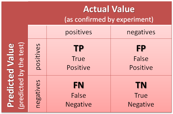
Let's consider a scenario where our observations consist of both positive (P) and negative (N) samples. The model provides two types of predictions: predicted positive (P') and predicted negative (N'). By analyzing these predictions, we can construct a confusion matrix as shown below:
 (Source: MathWorks)
In the confusion matrix, we have the following categories:
- True Positive (TP): Positive samples correctly predicted as positive.
- True Negative (TN): Negative samples correctly predicted as negative.
- False Positive (FP): Negative samples incorrectly predicted as positive.
- False Negative (FN): Positive samples incorrectly predicted as negative.
From the confusion matrix, we can observe the following relationships:
- P + N = Total number of observations.
- TP + TN = Number of true (correct) predictions.
- FP + FN = Number of false (incorrect) predictions.
- TP + FN = Total number of positive samples (P).
- TN + FP = Total number of negative samples (N).
- TP + FP = Total number of predicted positive samples (P').
- TN + FN = Total number of predicted negative samples (N').
Therefore, Accuracy (ACC) = (TP + TN)/(P + N)
We can derive 8 more useful metrics based on TP, FP, TN, FN. These are:
- Recall/Sensitivity/Hit Rate/True Positive Rate (TPR) = TP/P
- Miss Rate/False Negative Rate (FNR) = FN/P
- Specificity (SPC)/True Negative Rate (TNR) = TN/N
- Fall-out/False Positive Rate (FPR) = FP/N
- Precision/Positive predictive value (PPV) = TP/P'
- False Discovery Rate (FDR) = FP/P'
- Negative predictive value (NPV) = TN/N'
- False Omission Rate (FOR) = FN/N'
Further Derivations:
- Positive Likelihood ratio (LR+) = TPR/FPR
- Negative Likelihood ratio (LR-) = FNR/TNR
Sample Values:

Actual Predicted
1 1
0 0
0 1
1 0
1 1
0 0
0 0
1 0

Metrics:

P = 4
N = 4
P' = 3
N' = 5

TP = 2
TN = 3
FP = 1
FN = 2

P + N = 8
TP + TN = 5
FP + FN = 3
TP + FN = P = 4
TN + FP = N = 4
TP + FP = P' = 3
TN + FN = N' = 5
ACC = (TP + TN)/(P + N) = 5/8 = 0.625

Recall/TPR = TP/P = 2/4 = 0.5
FNR = FN/P = 2/4 = 0.5
TNR = TN/N = 3/4 = 0.75
FPR = FP/N = 1/4 = 0.25
Precision/PPV = TP/P' = 2/3 = 0.67
FDR = FP/P' = 1/3 = 0.33
NPV = TN/N' = 3/5 = 0.6
FOR = FN/N' = 2/5 = 0.4

LR+ = TPR/FPR = 0.5/0.25 = 2
LR- = FNR/TNR = 0.5/0.75 = 0.67
Another commonly used evaluation metric is AUC (Area under the curve)/ROC (Receiver operating characteristic) curve score.
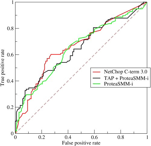
ROC Curve (Source:Wikipedia)
A ROC space is defined by FPR and TPR as x and y axes, respectively, which depicts relative trade-offs between true positive (benefits) and false positive (costs). The ROC curve is created by plotting the true positive rate (TPR) against the false positive rate (FPR) at various threshold settings. AUC is the area under the ROC Curve. A higher AUC score signifies a better model.